 11.2 等値面(isosurface)
isosurface {
  function { FUNCTION_ITEMS }
  [ contained_by { SPHERE | BOX } ]
  [ threshold FLOAT_VALUE ]
  [ accuracy FLOAT_VALUE ]
  [ max_gradient FLOAT_VALUE ]
  [ evaluate P0, P1, P2 ]
  [ open ]
  [ max_trace INTEGER ] | [ all_intersections ]
  [ OBJECT_MODIFIERS... ]
}
|
||
| isosurface | 等値面を指定するキーワード | |
| function { FUNCTION_ITEMS } | 等値面を定義する関数の指定 ⇒「11.2-5 関数」 | |
| contained_by { SPHERE | BOX } | 等値面を生成する範囲の指定、球またはボックスで指定する。[ディフォルト:box{-1,1} ] ⇒「11.2-1 生成範囲」 | |
| threshold FLOAT_VALUE | 等値面を生成するための値(閾値)の指定 [ディフォルト:0] ⇒「11.2-2 閾値」 | |
| accuracy FLOAT_VALUE | 再帰分割の値の指定、小さいほど正確な値が得られる。[ディフォルト:0.001] | |
| max_gradient FLOAT_VALUE | 関数の最大勾配の指定 [ディフォルト:1.1] ⇒「11.2-3 最大勾配関数」 | |
| evaluate P0, P1, P2 | 最大勾配を動的に探索する機能。P0は最小値、P1は最大値、P2は減衰値で指定する。 | |
| open | contained_byで指定された物体の形状を生成しない指定、等値面のみの生成となる。[ディフォルト:生成する] ⇒「11.2-4 オープン」 | |
| max_trace INTEGER | CSGにおける交差面のチェック回数の指定 | |
| all_intersections | CSGにおける交差面を全てチェックする。 | |
| OBJECT_MODIFIERS... | 変形などの指定 | |
11.2-1 生成範囲(contained_by)
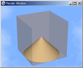 |
  isosurface {
    function { sqrt(pow(x,2) + pow(y,2)) + z }
    contained_by { box { -2, 2 } }
    max_gradient 1.8
    pigment{color rgb<1,0.88,0.65>}
  }
|
11.2-2 閾値(threshold)
        isosurface {
           function { sqrt(pow(x,2) + pow(y,2) + pow(z,2)) }
           contained_by { box { -2, 2 } }
           threshold 2
        }
        isosurface {
           function { sqrt(pow(x,2) + pow(y,2) + pow(z,2)) - 2 }
           contained_by { box { -2, 2 } }
        }
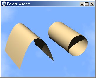
11.2-3 最大勾配(max_gradient)
 |
  //---------------Left
  isosurface {
     function { pow(x,2) + z - 0.5 }
     contained_by { box { -2, 2 } }
     max_gradient 3
     pigment{color rgb<1,0.88,0.65>}
     translate <2,0,1>
   }
  //---------------Right
  isosurface {
     function { pow(x,2) + z - 0.5 }
     contained_by { box { -2, 2 } }
     pigment{color rgb<1,0.88,0.65>}
     translate <-2,0,1>
   }
|
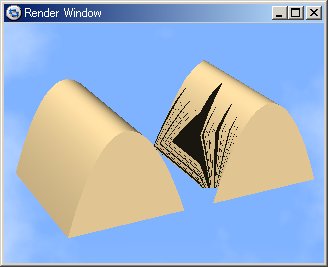
11.2-4 オープン(open)
 |
  //----------------Left
  isosurface {
    function { pow(x,2) + z - 0.5 }
    contained_by { box { -2, 2 } }
    max_gradient 3
    open
    pigment{color rgb<1,0.88,0.65>}
    translate <2,0,1>
  }
  //----------------Right
  isosurface {
    function { sqrt(pow(x,2) + pow(z,2)) - 1 }
    contained_by { box { -2, 2 } }
    max_gradient 3
    open
    pigment{color rgb<1,0.88,0.65>}
    translate <-2,0,0>
  }
|
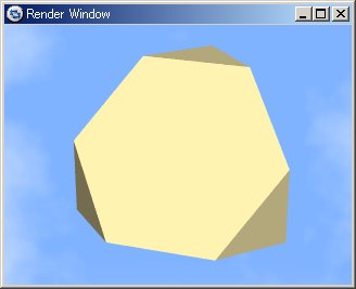
11.2-5 関数(function)
|
  isosurface {
    function { x + y + z }
    contained_by { box { -2, 2 } }
    max_gradient 1.8
    pigment{color rgb<0.8,0.75,0.55>}
  }
|
|
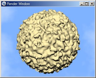
  isosurface {
     function { f_noise3d(x, y, z) - 0.5 }
    contained_by { box { -2, 2 } }
    max_gradient 1.8
    pigment{color rgb<0.8,0.75,0.55>}
  }
|
|
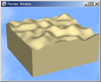
  isosurface {
    function { z + f_noise3d(x, y, 0) }
    contained_by { box { -3,3 } }
    max_gradient 1.8
    pigment{color rgb<0.8,0.75,0.55>}
  }
|
|
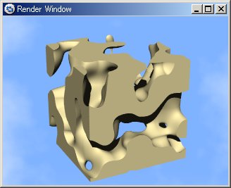
  isosurface {
    function { f_sphere(x, y, z, 1.6)
               - f_noise3d(x*5, y*5, z*5)*0.5 }
    contained_by { box { -2, 2 } }
    max_gradient 3
    pigment{color rgb<0.8,0.75,0.55>}
  }
|
11.2-6 関数の応用
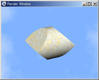
(a) 論理和: min 関数の使用
|
  #declare fn_A=function{sqrt(pow(y,2)+pow(z,2))-0.8}
  #declare fn_B=function{abs(x)+abs(z)-1}
  isosurface {
    function { min( fn_A(x,y,z), fn_B(x,y,z) ) }
    contained_by { box { -2, 2 } }
    max_gradient 1.8
    texture {T_Grnt1}
    scale 1.8
  }
|
(b) 論理積: max 関数の使用
|
  #declare fn_A=function{sqrt(pow(y,2)+pow(z,2))-0.8}
  #declare fn_B=function{abs(x)+abs(z)-1}
  isosurface {
     function { max( fn_A(x,y,z), fn_B(x,y,z) ) }
     contained_by { box { -2, 2 } }
     max_gradient 1.8
     texture {T_Grnt1}
         scale 1.8
  }
|
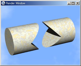
(c) 論理差: min 関数、引く関数に-をつける。
|
  #declare fn_A=function{sqrt(pow(y,2)+pow(z,2))-0.8}
  #declare fn_B=function{abs(x)+abs(z)-1}
  isosurface {
     function { max( fn_A(x,y,z), -fn_B(x,y,z) ) }
     contained_by { box { -2, 2 } }
     max_gradient 1.8
     texture {T_Grnt1}
     scale 1.8
  }
|
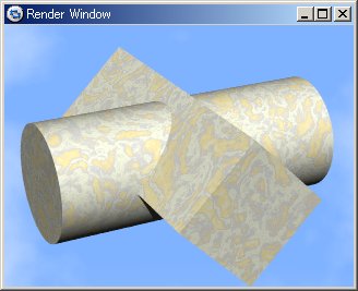
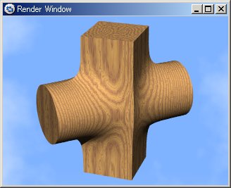
(d)ブロブ
|
  #declare fn_A=function{sqrt(pow(y,2)+pow(z,2))-0.8}
  #declare fn_C=function{abs(x)+abs(y)-1}
  #declare Blob_threshold=0.01;
  isosurface {
     function {
       1+Blob_threshold
          - pow( Blob_threshold, fn_A(x,y,z) )
          - pow( Blob_threshold, fn_C(x,y,z) )
      }
     contained_by { box { -2, 2 } }
     max_gradient 6
     texture {T_Wood7 scale 0.5}
     scale 1.4
  }
|